Getting Started with Arduino

What is Arduino?

Arduino is a tool for making computers that can sense and control more of the physical world than your desktop computer. It's an open-source physical computing platform based on a simple microcontroller board, and a development environment for writing software for the board.

Arduino can be used to develop interactive objects, taking inputs from a variety of switches or sensors, and controlling a variety of lights, motors, and other physical outputs. Arduino projects can be stand-alone, or they can be communicate with software running on your computer (e.g. Flash, Processing, MaxMSP.) The boards can be assembled by hand or purchased preassembled; the open-source IDE can be downloaded for free.

The Arduino programming language is an implementation of Wiring, a similar physical computing platform, which is based on the Processing multimedia programming environment.

Why Arduino?

There are many other microcontrollers and microcontroller platforms available for physical computing. Parallax Basic Stamp, Netmedia's BX-24, Phidgets, MIT's Handyboard, and many others offer similar functionality. All of these tools take the messy details of microcontroller programming and wrap it up in an easy-to-use package. Arduino also simplifies the process of working with microcontrollers, but it offers some advantage for teachers, students, and interested amateurs over other systems:

• Inexpensive - Arduino boards are relatively inexpensive compared to other microcontroller platforms. The least expensive version of the Arduino module can be assembled by hand, and even the pre-assembled Arduino modules cost less than $50
• Cross-platform - The Arduino software runs on Windows, Macintosh OSX, and Linux operating systems. Most microcontroller systems are limited to Windows.
• Simple, clear programming environment - The Arduino programming environment is easy-to-use for beginners, yet flexible enough for advanced users to take advantage of as well. For teachers, it's conveniently based on the Processing programming environment, so students learning to program in that environment will be familiar with the look and feel of Arduino
• Open source and extensible software- The Arduino software is published as open source tools, available for extension by experienced programmers. The language can be expanded through C++ libraries, and people wanting to understand the technical details can make the leap from Arduino to the AVR C programming language on which it's based. SImilarly, you can add AVR-C code directly into your Arduino programs if you want to.
• Open source and extensible hardware - The Arduino is based on Atmel's ATMEGA8  and ATMEGA168microcontrollers. The plans for the modules are published under a Creative Commons license, so experienced circuit designers can make their own version of the module, extending it and improving it. Even relatively inexperienced users can build the breadboard version of the module in order to understand how it works and save money.

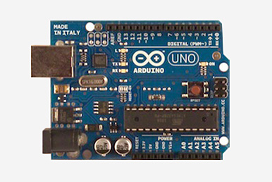
1 | Get an Arduino board and USB cable

We assume you're using an Arduino Uno, Arduino Duemilanove, Nano, Arduino Mega 2560 , or Diecimila. If you have another board, read the corresponding page in this getting started guide.

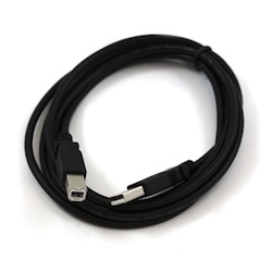
You also need a standard USB cable (A plug to B plug): the kind you would connect to a USB printer.

2 | Download the Arduino environment

Get the latest version from the download page.

When the download finishes, unzip the downloaded file. Make sure to preserve the folder structure. Double-click the folder to open it. There should be a few files and sub-folders inside.

3 | Connect the board

The Arduino Uno, Mega, Duemilanove and Arduino Nano automatically draw power from either the USB connection to the computer or an external power supply. If you're using an Arduino Diecimila, you'll need to make sure that the board is configured to draw power from the USB connection. The power source is selected with a jumper, a small piece of plastic that fits onto two of the three pins between the USB and power jacks. Check that it's on the two pins closest to the USB port.

Connect the Arduino board to your computer using the USB cable. The green power LED (labelled PWR) should go on.

4 | Install the drivers

Installing drivers for the Arduino Uno or Arduino Mega 2560 with Windows7, Vista, or XP:

·         Plug in your board and wait for Windows to begin it's driver installation process.  After a few moments, the process will fail, despite its best efforts

·         Click on the Start Menu, and open up the Control Panel.

·         While in the Control Panel, navigate to System and Security. Next, click on System. Once the System window is up, open the Device Manager.

·         Look under Ports (COM & LPT).  You should see an open port named "Arduino UNO (COMxx)"

·         Right click on the "Arduino UNO (COmxx)" port and choose the "Update Driver Software" option.

·         Next, choose the "Browse my computer for Driver software" option.

·         Finally, navigate to and select the driver file named "arduino.inf", located in the "Drivers" folder of the Arduino Software download (not the "FTDI USB Drivers" sub-directory). If you are using an old version of the IDE (1.0.3 or older), choose the Uno's driver file named "Arduino UNO.inf"

·         Windows will finish up the driver installation from there.

5 | Launch the Arduino application

Double-click the Arduino application. (Note: if the Arduino software loads in the wrong language, you can change it in the preferences dialog.)

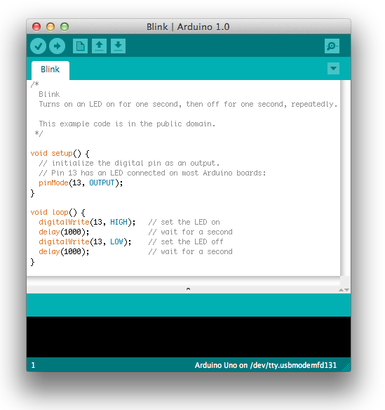
6 | Open the blink example

Open the LED blink example sketch: File > Examples > 1.Basics > Blink.

7 | Select your board

You'll need to select the entry in the Tools > Board menu that corresponds to your Arduino.

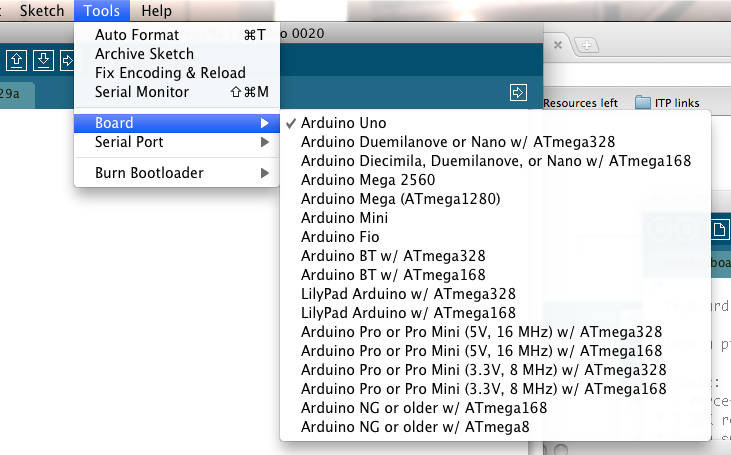
Selecting an Arduino Uno

For Duemilanove Arduino boards with an ATmega328 (check the text on the chip on the board), select Arduino Duemilanove or Nano w/ ATmega328. Previously, Arduino boards came with an ATmega168; for those, selectArduino Diecimila, Duemilanove, or Nano w/ ATmega168.

8 | Select your serial port

Select the serial device of the Arduino board from the Tools | Serial Port menu. This is likely to be COM3 or higher (COM1 and COM2 are usually reserved for hardware serial ports). To find out, you can disconnect your Arduino board and re-open the menu; the entry that disappears should be the Arduino board. Reconnect the board and select that serial port.

9 | Upload the program

Now, simply click the "Upload" button in the environment. Wait a few seconds - you should see the RX and TX leds on the board flashing. If the upload is successful, the message "Done uploading." will appear in the status bar. 

A few seconds after the upload finishes, you should see the pin 13 (L) LED on the board start to blink (in orange). If it does, congratulations! You've gotten Arduino up-and-running.

DEVELOPMENTS IN THE FIELD OF VLSI

There are a number of directions a person can take in VLSI, and they are all closely related to each other. Together, these developments are going to make possible the visions of embedded systems and ubiquitous computing.

1. Reconfigurable computing:
Reconfigurable computing is a very interesting and pretty recent development in microelectronics. It involves fabricating circuits that can be reprogrammed on the fly! And no, we are not talking about microcontrollers running with EEPROM inside. Reconfigurable computing involves specially fabricated devices called FPGA's, that when programmed act just like normal electronic circuits. They are so designed that by changing or "reprogramming" the connections between numerous sub modules, the FPGA's can be made to behave like any circuit we wish.

This fantastic ability to create modifiable circuits again opens up new possibilities in microelectronics. Consider for example, microprocessors which are partly reconfigurable. We know that running complex programs can benefit greatly if support was built into the hardware itself. We could have a microprocessor that could optimise itself for every task that it tackled! Or then consider a system that is too big to implement on hardware that may be limited by cost, or other constraints. If we use a reconfigurable platform, we could design the system so that parts of it are mapped onto the same hardware, at different times. One could think of many such applications, not the least of which is prototyping - using an FPGA to try out a new design before it is actually fabricated. This can drastically reduce development cycles, and also save some money that would have been spent in fabricating prototype IC's

2. Software Engineers taking over hardware design?:
ASIC's provide the path to creating miniature devices that can do a lot of diverse functions. But with the impending boom in this kind of technology, what we need is a large number of people who can design these IC's. This is where we realise that we cross the threshold between a chip designer and a systems designer at a higher level. Does a person designing a chip really need to know every minute detail of the IC manufacturing process? Can there be tools that allow a designer to simply create design specifications that get translated into hardware specifications?

The solution to this is rather simple - hardware compilers or silicon compilers as they are called. We know by now, that there exist languages like VHDL which can be used to specify the design of a chip. What if we had a compiler that converts a high level language into a VHDL specification? The potential of this technology is tremendous - in simple manner, we can convert all the software programmers into hardware designers!

3. The need for hardware compilers:
Before we go further let us look at why we need this kind of technology, that can convert high-level languages into hardware definitions. We see a set of needs which actually lead from one to the other in a series.

A. Rapid development cycles.
The traditional method of designing hardware is a long and winding process, going through many stages with special effort spent in design verification at every stage. This means that the time from drawing board to market, is very long. This proves to be rather undesirable in case of large expanding market, with many competitors trying to grab a share. We need alternatives to cut down on this time so that new ideas reach the market faster, where the first person to get in normally gains a large advantage.

B. Large number of designers.
With embedded systems becoming more and more popular, there is a need for a large number of chip designers, who can churn out chips designed for specific applications. Its impractical to think of training so many people in the intricacies of VLSI design.

C. Specialized training.
A person who wishes to design ASIC's will require extensive training in the field of VLSI design. But we cannot possibly expect to find a large number of people who would wish to undergo such training. Also, the process of training these people will itself entail large investments in time and money. This means there has to be system a which can abstract out all the details of VLSI, and which allows the user to think in simple system-level terms.

There are quite a few tools available for using high-level languages in circuit design. But this area has started showing fruits only recently. For example, there is a language called Handel-C, that looks just like good old C. But it has some special extensions that make it usable for defining circuits. A program written in Handel-C, can be represented block-by-block by hardware equivalents. And in doing all this, the compiler takes care of all low-level issues like clock-frequency, layout, etc. The biggest selling point is that the user does not really have to learn anything new, except for the few extensions made to C, so that it may be conveniently used for circuit design.

Another quite different language, that is still under development, is Lava. This is based on an esoteric branch of computer science, called "functional programming". FP itself is pretty old, and is radically different from the normal way we write programs. This is because it assumes parallel execution as a part of its structure - its not based on the normal idea of "sequence of instructions". This parallel nature is something very suitable for hardware since the logic circuits are is inherently parallel in nature. Preliminary studies have shown that Lava can actually create better circuits than VHDL itself, since it affords a high-level view of the system, without losing sight of low-level features.

HOW TO SELECT A MICRO CONTROLLER

 Choosing an MCU for your project is not easy.There are a large number of suppliers, offering varying architectures, peripherals, price points, power consumption, packages and what not. This article helps you get a better idea of the current situation and select the right MCU for your application.
A search in an online catalogue for microcontroller units (MCUs) would lead you to a massive collection of thousands upon thousands of various MCUs, leaving you spoilt for choice. There would be so many good choices that it would be difficult to make a decision. The following is what the experienced designers in the industry advise.

Architecture

            For most embedded systems you have the choice between 8-bit, 16-bit and 32-bit cores. When it comes to applications involving computations, 32-bit cores have a clear edge over 8-bit and 16-bit, in addition to making the most of the compiler features.
            The RISC and CISC architectures have become a little less meaningful with continued evolution of both the CISC and RISC designs and implementations. 
            The architecture of a microcontroller refers to the philosophy of the internal implementation, It includes details like how many registers are used, whether the code can execute out of the data memory, whether the peripherals are treated like memory, registers or something else, whether there is a stack and how it works, and so on. A RISC processor can handle simple math functions much faster, but a CISC processor will handle complicated functions faster because it can do them all at once instead of the several processing commands that a RISC processor would have to take to complete the same function.” MCU process technology, architecture and memory technology also need to be considered as these affect the real calculation speed rather than MHz and memory size requirements.

TOP 7 Factors to be Considered:-

 1.      8-bit vs 32-bit core. 8-bit cores are currently the most widely used MCU cores. For almost all tasks, an 8-bit core like 8051, PIC and AVR will suffice. However, as the project complexity increases, some may want to utilise the 32-bit cores like ARM, which provide you with more features and faster clock speeds but tend to have a higher learning curve than 8-bit cores. Some 32-bit cores also have floating-point units, which enable you to process math/DSP related functions faster and much more efficiently. However, you should get familiar with 8-bit cores before moving to 32-bit cores.

2.      Programming language. This is indirectly related to the MCU but directly to the tool chain used. The most popular programming languages for MCUs are Assembly (ASM) and Embedded C.
Working with ASM is much more time-consuming but gives you great insight into the architecture and actual working of the MCU. However, when the code size efficiency does not matter as much as the time to develop, Embedded C is the way to go. Again, you can write efficient code in ‘C’ and some projects require you to use ‘C’ to keep things simple.
For most of the 8051s available in the Indian market, Keil supports the code in ASM and Embedded C. For the PIC series, MPLAB has a CCS plugin (I use this as opposed to Hi-Tech Compiler), which enables you to code a PIC in ‘C’. So before you select the chip, make sure a tool chain with the right options is available for development. Do consider the cost of the same as many of them do not have free versions.

3.       GPIOs and features. Manufacturers release many MCUs of similar specifications but different features and resolutions. Select a chip that has all the features with the resolution as per your needs. Try to keep external chip interfacing to a minimum. This will help you in your design. Also make sure your MCU has sufficient input/output (I/O) pins for your needs. Try using alternate modes for peripherals—like 4-bit LCD mode—to save some I/O pins.

4.       Cost. If it is your first time working with an MCU, there is no need to purchase an expensive MCU. We all have had our share of burnt MCUs, and likely you will too. So keep the cost low initially. Weigh all the points mentioned here (and elsewhere too) and select an appropriately priced MCU that suits your budget. For absolute beginners,  I would recommend AT89S series and P89V51RD2 (expensive but has PWMs) from 8051 family, and PIC16F877A (has ADCs too) from PIC family. In general, 8051s tend to be cheaper than PICs, which are cheaper than Atmega’s, but PICs have much more functionality.

5.      Availability. Select an MCU that will be available for a long time to come. There is no general rule of thumb to know this, but selecting a popular one is your best bet. (The ones mentioned above are most widely used in many universities.) If for some reason you select an MCU which is not available in India, you may have to pay additional shipping charges to get it, which will be costly as well as frustrating.

6.      Online support. This is crucial when you’re just venturing out and when you move on to 32-bit cores. Selecting an MCU which has good online support will help you with your ideas and solve most of your problems as the experience of other users is available for your reference. Getting to know existing bugs with tool chains or MCU documentation will help you avert the problem in advance and speed up development.

7.      Packaging. For most DIY projects, a DIP package is suitable and easy to work with. SMD packages are a bit difficult to work with without proper tools and therefore not recommended for first timers. Once the design is ready, you can always use SMD equivalents to make it more compact.

Operational amplifier (op-amp)

An operational amplifier (op-amp) is a DC-coupled high-gain electronic voltage amplifier with a differential input and, usually, a single-ended output. In this configuration, an op-amp produces an output potential (relative to circuit ground) that is typically hundreds of thousands of times larger than the potential difference between its input terminals.

Operational amplifiers had their origins in analog computers, where they were used to do mathematical operations in many linear, non-linear and frequency-dependent circuits. Characteristics of a circuit using an op-amp are set by external components with little dependence on temperature changes or manufacturing variations in the op-amp itself, which makes op-amps popular building blocks for circuit design.

Op-amps are among the most widely used electronic devices today, being used in a vast array of consumer, industrial, and scientific devices. Many standard IC op-amps cost only a few cents in moderate production volume; however some integrated or hybrid operational amplifiers with special performance specifications may cost over $100 US in small quantities. Op-amps may be packaged as components, or used as elements of more complex integrated circuits.

The op-amp is one type of differential amplifier. Other types of differential amplifier include the fully differential amplifier (similar to the op-amp, but with two outputs), the instrumentation amplifier (usually built from three op-amps), the isolation amplifier (similar to the instrumentation amplifier, but with tolerance to common-mode voltages that would destroy an ordinary op-amp), and negative feedback amplifier (usually built from one or more op-amps and a resistive feedback network).

Circuit Notation

The circuit symbol for an op-amp is shown to the right, where:

• V₊: non-inverting input
• V₋: inverting input
• V_out: output
• V_S+: positive power supply
• V_S−: negative power supply

The power supply pins (V_S+ and V_S−) can be labeled in different ways. Often these pins are left out of the diagram for clarity, and the power configuration is described or assumed from the circuit.

OPERATION

The amplifier's differential inputs consist of a V₊ input and a V₋ input, and ideally the op-amp amplifies only the difference in voltage between the two, which is called the differential input voltage. The output voltage of the op-amp is given by the equation:

where V₊ is the voltage at the non-inverting terminal, V₋ is the voltage at the inverting terminal and A_OL is the open-loop gain of the amplifier (the term "open-loop" refers to the absence of a feedback loop from the output to the input).

The magnitude of A_OL is typically very large—100,000 or more for integrated circuit op-amps—and therefore even a quite small difference between V₊and V₋ drives the amplifier output nearly to the supply voltage. Situations in which the output voltage is equal to or greater than the supply voltage are referred to as saturation of the amplifier. The magnitude of A_OL is not well controlled by the manufacturing process, and so it is impractical to use an operational amplifier as a stand-alone differential amplifier. Without negative feedback, and perhaps with positive feedback for regeneration, an op-amp acts as a comparator. If the inverting input is held at ground (0 V) directly or by a resistor, and the input voltage V_in applied to the non-inverting input is positive, the output will be maximum positive; if V_in is negative, the output will be maximum negative. Since there is no feedback from the output to either input, this is an open loop circuit acting as a comparator. The circuit's gain is just the A_OL of the op-amp.

If predictable operation is desired, negative feedback is used, by applying a portion of the output voltage to the inverting input. The closed loop feedback greatly reduces the gain of the amplifier. When negative feedback is used, the circuit's overall gain and response becomes determined mostly by the feedback network rather than by the op-amp itself. If the feedback network is made of components with relatively constant, stable values, the variability of the op-amp's open loop response does not seriously affect the circuit's performance. The response of the op-amp circuit with its input, output and feedback circuits to an input is characterized mathematically by a transfer function. Designing an op-amp circuit to have a desired transfer function is in the realm of electrical engineering. The transfer functions are important in most applications of op-amps, such as in analog computers. High inputimpedance at the input terminals and low output impedance at the output terminal(s) are particularly useful features of an op-amp.

For example, in a non-inverting amplifier (see the figure on the right) adding a negative feedback via the voltage divider R_f, R_g reduces the gain. Equilibrium will be established when V_out is just sufficient to reach around and "pull" the inverting input to the same voltage as V_in. The voltage gain of the entire circuit is determined by 1 + R_f/R_g. As a simple example, if V_in = 1 V and R_f = R_g, V_out will be 2 V, the amount required to keep V₋ at 1 V. Because of the feedback provided by R_f, R_g this is a closed loop circuit. Its overall gain V_out / V_in is called the closed-loop gain A_CL. Because the feedback is negative, in this case A_CL is less than the A_OL of the op-amp.

Another way of looking at it is to make two relatively valid assumptions.

One, that when an op-amp is being operated in linear (not saturated) mode, the difference in voltage between the non-inverting (+) pin and the inverting (−) pin is so small as to be considered negligible

The second assumption is that the input impedance at both (+) and (−) pins is extremely high (at least several megohms with modern op-amps).

Thus, when the circuit to the right is operated as a non-inverting linear amplifier, V_in will appear at the (+) and (−) pins and create a current i through R_g equal to V_in/R_g. Since Kirchhoff's current law states that the same current must leave a node as enter it, and since the impedance into the (−) pin is near infinity, we can assume the overwhelming majority of the same current i travels through R_f, creating an output voltage equal to V_in + i × R_f. By combining terms, we can easily determine the gain of this particular type of circuit.

CHARACTERISTICS 

Real operational amplifiers suffer from several non-ideal effects:

Finite gain

Open-loop gain is infinite in the ideal operational amplifier but finite in real operational amplifiers. Typical devices exhibit open-loop DC gain ranging from 100,000 to over 1 million. So long as the loop gain (i.e., the product of open-loop and feedback gains) is very large, the circuit gain will be determined entirely by the amount of negative feedback (i.e., it will be independent of open-loop gain). In cases where closed-loop gain must be very high, the feedback gain will be very low, and the low feedback gain causes low loop gain; in these cases, the operational amplifier will cease to behave ideally.

Finite input impedances
The differential input impedance of the operational amplifier is defined as the impedance between its two inputs; the common-mode input impedance is the impedance from each input to ground. MOSFET-input operational amplifiers often have protection circuits that effectively short circuit any input differences greater than a small threshold, so the input impedance can appear to be very low in some tests. However, as long as these operational amplifiers are used in a typical high-gain negative feedback application, these protection circuits will be inactive. The input bias and leakage currents described below are a more important design parameter for typical operational amplifier applications.

Non-zero output impedance
Low output impedance is important for low-impedance loads; for these loads, the voltage drop across the output impedance of the amplifier will be significant. Hence, the output impedance of the amplifier limits the maximum power that can be provided. In configurations with a voltage-sensing negative feedback, the output impedance of the amplifier is effectively lowered; thus, in linear applications, op-amps usually exhibit a very low output impedance indeed. Negative feedback can not, however, reduce the limitations that R_load in conjunction with R_out place on the maximum and minimum possible output voltages; it can only reduce output errors within that range.
Low-impedance outputs typically require high quiescent (i.e., idle) current in the output stage and will dissipate more power, so low-power designs may purposely sacrifice low output impedance.

Input current
Due to biasing requirements or leakage, a small amount of current (typically ~10 nanoamperes for bipolar op-amps, tens of picoamperes for JFET input stages, and only a few pA for MOSFET input stages) flows into the inputs. When large resistors or sources with high output impedances are used in the circuit, these small currents can produce large unmodeled voltage drops. If the input currents are matched, and the impedance looking out of both inputs are matched, then the voltages produced at each input will be equal. Because the operational amplifier operates on the difference between its inputs, these matched voltages will have no effect (unless the operational amplifier has poor CMRR, which is described below). It is more common for the input currents (or the impedances looking out of each input) to be slightly mismatched, and so a small offset voltage (different from the input offset voltage below) can be produced. This offset voltage can create offsets or drifting in the operational amplifier. It can often be nulled externally; however, many operational amplifiers include offset null or balance pins and some procedure for using them to remove this offset. Some operational amplifiers attempt to nullify this offset automatically.

Input offset voltage
This voltage, which is what is required across the op-amp's input terminals to drive the output voltage to zero,^{[6][nb 1]} is related to the mismatches in input bias current. In the perfect amplifier, there would be no input offset voltage. However, it exists in actual op-amps because of imperfections in the differential amplifier that constitutes the input stage of the vast majority of these devices. Input offset voltage creates two problems: First, due to the amplifier's high voltage gain, it virtually assures that the amplifier output will go into saturation if it is operated without negative feedback, even when the input terminals are wired together. Second, in a closed loop, negative feedback configuration, the input offset voltage is amplified along with the signal and this may pose a problem if high precision DC amplification is required or if the input signal is very small.^{[nb 2]}

Common-mode gain
A perfect operational amplifier amplifies only the voltage difference between its two inputs, completely rejecting all voltages that are common to both. However, the differential input stage of an operational amplifier is never perfect, leading to the amplification of these identical voltages to some degree. The standard measure of this defect is called the common-mode rejection ratio(denoted CMRR). Minimization of common mode gain is usually important in non-inverting amplifiers (described below) that operate at high amplification.
Output sink current
The output sink current is maximum current allowed to sink into the output stage. Some manufacturers show the output voltage vs. the output sink current plot, which gives an idea of the output voltage when it is sinking current from another source into the output pin.
Temperature effects
All parameters change with temperature. Temperature drift of the input offset voltage is especially important.

Power-supply rejection
The output of a perfect operational amplifier will be completely independent from ripples that arrive on its power supply inputs. Every real operational amplifier has a specified power supply rejection ratio (PSRR) that reflects how well the op-amp can reject changes in its supply voltage. Copious use of bypass capacitors can improve the PSRR of many devices, including the operational amplifier.

Drift
Real op-amp parameters are subject to slow change over time and with changes in temperature, input conditions, etc.

Noise
Amplifiers generate random voltage at the output even when there is no signal applied. This can be due to thermal noise and flicker noise of the devices. For applications with high gain or high bandwidth, noise becomes a very important consideration.

Classification of Microcontrollers

A microcontroller is a small computer on a single integrated circuit containing a processor core, memory, and programmable input/output peripherals. Program memory in the form of NOR flash or OTP ROM is also often included on chip, as well as a typically small amount of RAM.

Types of Microcontroller:

The microcontrollers are characterized regarding bus-width, instruction set, and memory structure. This article is going to describe some of the basic types of the Microcontroller that newer users may not know about. So the microcontroller can be classified according to their charecteristics as shown in graph below:

Bits:

• The bits in microcontroller are 8-bits, 16-bits and 32-bits microcontroller.In 8-bit microcontroller, the point when the internal bus is 8-bit then the ALU is performs the arithmetic and logic operations. The examples of 8-bit microcontrollers are Intel 8031/8051, PIC1x and Motorola MC68HC11 families.
• The 16-bit microcontroller performs greater precision and performance as compared to 8-bit. For example 8 bit microcontrollers can only use 8 bits, resulting in a final range of 0×00 – 0xFF (0-255) for every cycle. In contrast, 16 bit microcontrollers with its 16 bit data width has a range of 0×0000 – 0xFFFF (0-65535) for every cycle. A longer timer most extreme worth can likely prove to be useful in certain applications and circuits. It can automatically operate on two 16 bit numbers. Some examples of 16-bit microcontroller are 16-bit MCUs are extended 8051XA, PIC2x, Intel 8096 and Motorola MC68HC12 families.
• The 32-bit microcontroller uses the 32-bit instructions to perform the arithmetic and logic operations. These are used in automatically controlled devices including implantable medical devices, engine control systems, office machines, appliances and other types of embedded systems. Some examples are Intel/Atmel 251 family, PIC3x.

Memory/Devices:

Embedded microcontroller: When an embedded system has an MCU that has all the hardware and software units in a single unit, the MCU is called embedded microcontroller. Very few or no other external unit or system is present for processing during the control or use of the external devices. For example, a telephone handset circuit uses an embedded microcontroller.

External memory microcontroller: When an embedded system has an MCU that has all the hardware and software units present not as a single unit and has all or part of the memory unit externally interfaced using an interfacing circuit which is called the glue circuit, the MCU is called an external memory microcontroller. For example, 8031 has the program memory which is interfaced externally to it. The 8051 has both internal as well as external program memory.

Family:

The microcontrollers can also be classified according to their family. family is usually a company or a manufacturer in which controller is fabricated. Each family have its own architecture and instruction set. some though 8051 is famous but PIC and ARM are going more popular than 8051.

Instruction Set:

Complicated Instruction Set Computer (CISC) architecture microcontroller: When an MCU has an instruction set that supports many addressing modes for the arithmetic and logical instructions and when there are the memory accesses during the ALU operations and the data transfer instructions, the MCU is said to be possessing CISC-architecture.

CISC provides flexibility in choosing various ways of performing the data transfer, arithmetic and other operations. For example, it is feasible to add contents of two registers or add the register and memory or add the bits at two memory addresses in a CISC. Instructions are of variable number of bytes in the CISC. These can take varying amounts of time interval for execution. An example is Intel 8096.

Reduced Instruction Set Computer (RISC) microcontroller: When an MCU has an instruction set that supports a few addressing modes for the arithmetic and logical instructions and just a few (load, store, push and pop) instructions for the data transfer, the MCU is said to be of RISC architecture. RISC provides no flexibility in choosing the many different ways of performing the arithmetic and logic operations. These operations are performed after the load of operands in the registers, and the results of these operations are placed in registers. The register contents are later on stored in the memory. RISC implements each instruction in a single cycle using a distinct hardwired control. It uses a lesser amount of circuitry. It has less power dissipation. There is reduced instruction set. Instructions are of fixed number of bytes and take a fixed amount of time for execution. It has many registers. Therefore, operations can be performed using them. The need for external fetches from the memories are greatly reduced. (An external fetch is to be done by the CPU for an operand more frequently in the CISC). The RISC provides a higher performance in computing than the CISC. This is because little need of the external fetches, which takes a significant amount of processor time. High performance is also because of hardwired implementation of instructions. An example of RISC architecture is the ARM processor family-based MCU

Memory Architecture:

• Harvard Memory Architecture Microcontroller: The point when a microcontroller unit has a dissimilar memory address space for the program and data memory, the microcontroller has Harvard memory architecture in the processor.
• Princeton Memory Architecture Microcontroller: The point when a microcontroller has a common memory address for the program memory and data memory, the microcontroller has Princeton memory architecture in the processor.

This is how the MICs are classified, there may be some other types but most of the types can be seen through this major classification.

Basics of Matlab & its programming.

MATLAB is an integrated environment that is used for solving many problems in scientific domain. MATLAB is an abbreviation of the word – Matrix Laboratory. It is designed to perform matrix operations. Since images are 2D and 3D in nature, MATLAB is suitable for performing image manipulations. It is a powerful tool and can be used to implement imaging projects effectively. MATLAB package comes with several functions that facilitate the image processing. The power of MATLAB comes with a set of functions called toolboxes. A toolbox is a collection of functions that are designed to do image processing. Using these functions it is easier to load, save, and perform custom functions on images. The image processing toolbox allows us to do various tasks such as 

1.      Reading/ Writing of images

2.      Colour space and format conversions

3.      Visualization of images

4.      Image filtering

5.      Image Transforms

6.      Image arithmetic

7.      Morphological operations

MATLAB also comes with toolboxes for statistics, Wavelet, Neural networks. Apart from the official toolboxes, many public domain toolboxes are available to perform various tasks.

The subsequent sections discuss some of the basic programming capability of MATLAB.

Basics of MATLAB

Based on the versions of MATLAB, the visual appearance of MATLAB varies. But essentially the MATLAB environment has three basic windows.

1. Command Windows – In this main window, the MATLAB command prompt is >>. MATLAB is an interactive environment. The commands can be given one by one and can see the execution interactively. While this acceptable for simple scripts, for length programs this is not acceptable. To facilitate the project development, MATLAB provides an interactive environment window called Edit Window.
2. Edit Window – In this window, the programs can be written. The programs can be entered, edited and executed in this window. One can create programs with .m extension, called ‘M-files’. One can compare this with C program or Java program. A M-file is a collection of programming commands just like C programs to accomplish a task.
3. Graphics Window – This is the window used to visualize the graphics that are created in the MATLAB programs. This window also provides help to manipulate the figures such as changing the labels for axes, titles and for exporting the graphics.

MATLAB comes with lot of on-line help – Commands such as helpdesk, help, lookfor and helpwin to locate the context oriented help.

Data Types

The Fundamental data type of MATLAB is an array. Since images are matrices, MATLAB is a perfect fit for manipulating images. Apart from array, the MATLAB also supports many data types such as integers, double (including floating point numbers), character strings, structures and cells.

File Types

MATLAB provides three types of files.

M-Files – These are flat Ascii files that can be created using MATLAB environment or any other text editors. M-files are collection of MATLAB commands. There are two types of M-files.

            1. Script Files

            2. Function Files

Mat-Files – These are native data files with .mat extension. These are binary data that is created with the command save in the command prompt. In the next session, the data can be loaded with the command load. The advantage is that this is a special format that can be read only with MATLAB.

Mex-File – These are programs that can call other programming files that are written in programming languages like C or Fortran.

MATLAB can be launched by double-clicking the MATLAB icon or by navigating the MATLAB program.

Some simple commands like this can be tested

                        >> 2 + 4

MATLAB promptly returns the result. Instead of typing the MATLAB commands one by one, a set of valid MATLAB commands can be put into a file with .m extension. This is called script file. The script file can be executed in the command prompt by typing the file name. Caution should be taken that the scripts that are created by us should have a name that is different from the key words of MATLAB.

Function files are similar to script files. The main difference is all the variables defined in a function file are local. One can compare the function file with the function or subroutine of a programming language.

The structure of    a function file is given as

function [out_variables] = function_name (Input_parameters)

% First comment – This appears when the on-line help is sought called h1 line

% This symbol is an indication of comments that are used for documentation Statement(s).

As the structure is given above, functions are created with the keyword function   followed by the output variables. The definition of a function includes function name also with the necessary input arguments. The first line is called h1 line which is used to provide the comments that are useful to understand the reason for creating that function. This can be followed by many comments. Comments are useful to document the problem so that the third person can understand it. The core part of the function is a set of commands that are necessary to execute it.

Once a function is defined, the function can be executed by invoking it either by calling the function with or without the output variables. If the objective of the function is to display a graph, then storing the resultant may not be necessary. In that case, the output variables can be ignored.      

The functions can be called within another function also as

            t1 = @sample_function

Here a handle t1 is created for a sample function. This can be used inside for another function as

            t2 = sample_function2(t1,input_variables)

                                    or

            t2 = samplefunction2(@sample_function,input_variables)

This command is very useful in image processing for block processing.

To increase the speed of execution, the functions can be compiled readily. So the function is interpreted and translated to an intermediate form and stored for later uses. This approach increased the fastness. Also parsing creates a file that is in protected form. This is immensely useful to protect the identity of the programming code so that no one else can see the code and alter it.

MATLAB Programming language

Like any programming language like C or C++, MATLAB uses a set of programming constructs. This covers all the programming aspects like sequence, branching and repetition. Like other programming languages the global variables can be created with the command global.

  For example, the statement  

global  m,n

creates two global variables.

MATLAB provides branching using if-elseif-else statements as

                                    if condition1

                                       statement(s)

                                   else if condition2

                                       statement(s)

                                   else

   statement(s)

                                   end

Like C language, the conditions are executed and a logical branching is done. Based on the truth of the conditions the statements are executed. Else- Part is executed when both the conditions are false. When conditions become more, writing a recursive if statements with more conditions makes program difficult to understand. In that case the ‘switch’ statement is very helpful. The syntax for switch is given as

                                    switch indicator

                                    case value1

                                            Statement(s)

                                    case value2

                                            Statement(s)

                                    otherwise

                                           Default statement(s)

                                    end

Similarly MATLAB provides two repetitive statements for and while. The syntax for the statement for is given as

                                    for counter:=start:Increment:End

                                                statement(s)

                                    End

The increment can be positive or negative also. Initially the counter value is the start. then based on the increment , the counter value is incremented. Once it reaches the end value, the program control comes out of the loop. The statements are thus executed as per the start, end and increment value.

Similarly the statement ‘while’ can be used to execute a set of statements till the condition specified by the while is no longer satisfied. The syntax for ‘while’ statement is given as

                        while Condition

                                    Statement(s)

                        end

Other statements that are useful are

            1. Break – This statement is useful break out of a loop in a loop. This is applicable even if the condition of the execution is true.

            2. Return – This statement simply returns the program control to the function that invokes it.

            3. error – When there is a problem inside a function or script, this statement is useful for returning the control to the keyboard.

            4. pause – This statement is useful to temporarily pause or halt the current process and waits for the user response. pause(n) cause the ‘pause’ command  to last n seconds and resume after that.

Input Commands

The syntax of the input command is

                        output_variable = input(‘String’)

For example, the command   n = input(‘Enter the value of n’) display the string in the command prompt expecting the user response. The user response is collected and stored in the variable ‘n’.

When the choices are more, the command ‘menu’ can be used. The syntax of the command ‘menu’ is given as follows.

menu(‘Menu name’,’choice 1’, ‘choice 2’,….’choice n’)

This command creates an onscreen menu. Based on the response given by the user either by mouse or keyboard, the respective commands can be used. MATLAB provides advanced versions of GUI. One can use ‘menu’ command for some primitive level usage.

When the data becomes more, the files can be used. One can compare this with C programming language and some of its commands are shown below

1. fpen – Open a file or create a new file.

2. fclose – Close the file

3. fread – read the value from the file

4. fwrite – write the value into the file

5. fscanf – read the formatted data

6. fwritef – write the formatted data